In quantum mechanics, to describe the particle or particles in space we use wave functions, which we can describe as the superposition of the basis functions.
Example of quantum state of the order o=5 in one point described by radius vector \(\vec{
r}\) from the nucleus:
\(\psi(r) = c_{1}\Phi_{1}(r) +c_{2} \Phi_{2}(r) + c_{3} \Phi_{3}(r) +c_{4}\Phi_{4}(r)+ c_{5}\Phi_{5}(r) \quad \quad \quad (1)\).
Weights here are \(c_{1} - c_{5}\). If basis function are orthonormal, we get these weights in the range <0,1> as the eigenvector by solving eigenvalue problem \(\hat{H} \Psi(r) = E \Psi(r) \).
Basis functions describe whole space interval, one possibility to make atom/molecule basis functions in 1-D are B-splines (Basis - splines). B-splines are defined in the restricted space compare to Slater or Gaussians orbitals.
So first, let's define the box [a b]:
a=0;
b=500;
Number of discrete steps defines vector of breakpoints:
dX=(b-a)/(N_b-1);
x_break=a:dX:b;
Number of B-splines, Nb, must be at least twice the length of the box b.
Nb=1000
B-splines are spanned on the whole box. Except of breaking points we define also knot-points. Each B-spline is starting on the each knot-points. Number of knot points = Number of B-splines. You can set up knot sequence as you like.
In our case, knot points are equal to the breaking points except on the boundaries, where the multiplicity of knot-points is the order of B-splines o+1. Also the degree of polynomials is defined as o+1.
In our case, the order is o=5. This order also define the number of control points for each splines between two knot-points.
Plot(1)
On the plot above Plot(1) are B-splines of the order o=5. You can see number of control points between each adjacent knot points is equal to the order of B-splines. Notice that at the boundary you have multiplicity of knot-points equals to of the o+1, therefore o+1 B-splines are raising from the boundary point. Notice that B-spline spreads among knot points which number equals to the order of B-splines.
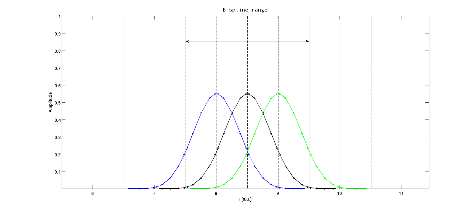
Plot(2)
Spreading of B-splines of order o=5 in the interval within 5 knot-points. Line '--' highlights each knot point.
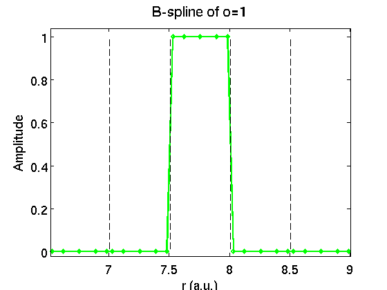
Plot(3)
Spreading of B-splines of order o=1 in the interval within 2 knot-points. Line '--' highlights
each knot point.
B-splines are given by recurrence relation
\[B_{i}^{o+1}(x)=\frac{x - t_{i}}{t_{i+o}-t_{i}}B_{i}^{o}(x) + (\frac{t_{i+o+1}-x}{t_{i+o+1} - t_{i+1}}) B_{i+1}^{o}(x) \quad \quad \quad (2)\].
where \(B_{i}^{o}\) is the B-spline starting on the
i-th knot-point
t, of the order o.
Each B-spline has the non-zero amplitude in the interval between neighboring knot points:
\[B_{i}^{o}(x)=\bigg\{
\frac{>0}{0} \frac{\textbf{if} \quad t_{i}\le x < t_{i+o} } {elsewise}\]
Be awared that you use only the B-splines of the highest order from the above reccurence equation to use it as the first approximation of eigenstates or other application. The order of splines must be at least o=4.
Each control point of the B-splines has its weight (see amplitude of the B-splines).
We get all control points (integration points) and its weight by the Golub-Welsch algorithm for first:
%%%%%%%%%%%%%%%%%%%%%%%%%%%%%%%%%%%%
%%Gauss-Legendre integration points and its weights%%%%%%%%%
%%%%%%%%%%%%%%%%%%%%%%%%%%%%%%%%%%%%
%o =5, is order of each B-spline
i=1:o;
B=1./2./sqrt(1-(2.*i).^(-2));
J(1:o,1:o)=0;
for j=1:n-1
J(j,j+1)=B(j);
J(j+1,j)=B(j);
end
[V,D] = eig(J);
for j=1:o
WW(j)=2.*V(1,j).^2;
%%%And control points are given by diagonalization:
xx(j)=D(j,j);
end
%%%%%%%%%%%%%%%%%%%%%%%%%%%%%%%%%%%%%%%%%%%%%%%%
Now we spread our controls points with corresponding weights on the whole interval defined by the breaking points x_breaks. Please notice that each spline has 5 control points between each two break points.
%Nb is number of B-splines on the whole interval
for i=2:Nb
x((i-2)*o+1:(i-1)*o)=(x_break(i)-x_break(i-1))./2.*xx+(x_break(i)+x_break(i-1))./2;
W((i-2)*o+1:(i-1)*o)=WW;
end
%%%%%%%%%%%%%%%%%%%%%%%%%%%%%%%%%%%%%%%%%%%%%%%%
Some application:
Control points define the integration points (as well for differentiate interval).
Kinetic Energy Matrix Operator with our basis function B:
Integral 1=-1./2.*dX./2.*sum(
W'.*B(:,i+1,o+1).*
diff_B(:,j+1,o+1));
H(i,j)=H(i,j)+int1;
To remind you: i=j. The size of Hamiltonian matrix is Nb x Nb of the order o. Differentiate of B-splines, diff_B, is given by recurrence relation:
\[\frac{d}{dx}B_{i}^{o+1}(x) = \frac{o (o-1)}{t(i+o)-t(o)}.\frac{B_{i}^{o-1}(x)}{t(i+o-1)-t(i)} - \frac{B_{i+1}^{o-1}(x)}{t(i+o)-t(i+1)} \\
- \frac{o (o-1)}{t(i+o-1)-t(i)}(\frac{B_{i+1}^{o-1}(x)}{t(i+o)-t(i+1)} - \frac{B_{i+2}^{o-1}(x)}{t(i+o+1)-t(i+2)}) \quad \quad \quad (3)\].
Because B- splines are
not orthogonal function, we need to compute the overlap matrix:
%S is overlap Matrix
int2=dX./2.*sum(
W'.*
B(:,i+1,o+1).*B(:,j+1,o+1));
S(i,j)=S(i,j)+int2;
After diagonalization, in matlab: [V,E] = eig(H,S), where V is the eigenstates vector, so we have new weights given by the vector V instead of initial W gained by Golub-Welsch algorithm for each B-spline in the box [a b]. E are the eigenvalues on diagonal.
We construct the state functions psi(r,i) as in the equation (1):
psi(:,i)=psi(:,i)+
V(j,i).*B(:,j+1,n+1)
j are the number of the B-splines Nb. For each state
i you need Nb basis functions \[\Phi(r)]\, only some of them are non-zero. The number of the states
i is given by the principal and angular quantum number (in this 1D case magnetic quantum number m=0). The size of
V(j,j) is Nb x Nb (as large as the Hamiltonian), maximum number of the states is Nb spread on Nb points.
To summarize basic charecteristics of B-splines as the state function:
Advantages:
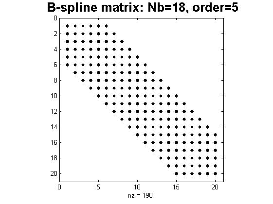
- sparse Hamiltonian matrix with (Nb-1)*(2*o+1)= non-zero elements. Very compact Hamiltonian is the excellent preconditions to use it in the time propagator to solve Time Dependent Schroedinger Equation (TDSE).
- low RAM consumption
- easily diagonalisable
Disdvantages:
- Not orthogonal, need to compute overlap matrix with make (2*(o+1)*Nb) nonzero elements
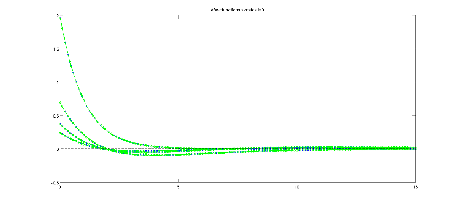
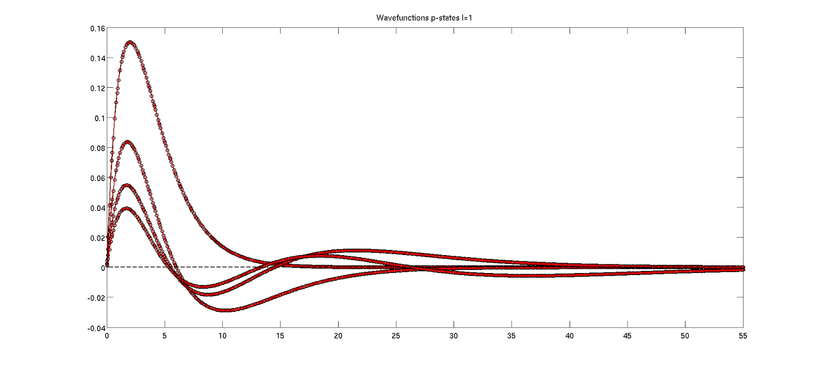
- They are not eigenfunctions of Hamiltonian. However wavefunctions at the small distance r from nucleus are the same as the analytical solution for hydrogen, which is showed at the plot below.
Plot(4) -Energy spectrum of the Hamiltonian in B-spline basis.
Plot(5)
For p-states red color radial wavefunctions are analytical solutions for hydrogen (
Slater-type function from http://en.citizendium.org/wiki/Hydrogen-like_atom), black color wavefunctions are generated in the basis of B-splines.
To make 3D wave function $\Psi(r,\Theta,\Phi)$, multiply $\Psi(r)$ with Legendre polynomial.